C4W2: Predicting time series
Contents
C4W2: Predicting time series#
https-deeplearning-ai/tensorflow-1-public/C4/W2/assignment/C4W2_Assignment.ipynb
Commit
50a14a4on Feb 6, 2023 - Compare
import numpy as np
import tensorflow as tf
import matplotlib.pyplot as plt
from dataclasses import dataclass
Generating the data#
def plot_series(time, series, format="-", start=0, end=None):
    plt.plot(time[start:end], series[start:end], format)
    plt.xlabel("Time")
    plt.ylabel("Value")
    plt.grid(False)

def trend(time, slope=0):
    return slope * time

def seasonal_pattern(season_time):
    """Just an arbitrary pattern, you can change it if you wish"""
    return np.where(season_time < 0.1,
                    np.cos(season_time * 6 * np.pi),
                    2 / np.exp(9 * season_time))

def seasonality(time, period, amplitude=1, phase=0):
    """Repeats the same pattern at each period"""
    season_time = ((time + phase) % period) / period
    return amplitude * seasonal_pattern(season_time)

def noise(time, noise_level=1, seed=None):
    rnd = np.random.RandomState(seed)
    return rnd.randn(len(time)) * noise_level
def generate_time_series():
# The time dimension or the x-coordinate of the time series
time = np.arange(4 * 365 + 1, dtype="float32")
# Initial series is just a straight line with a y-intercept
y_intercept = 10
slope = 0.005
series = trend(time, slope) + y_intercept
# Adding seasonality
amplitude = 50
series += seasonality(time, period=365, amplitude=amplitude)
# Adding some noise
noise_level = 3
series += noise(time, noise_level, seed=51)
return time, series
# Save all "global" variables within the G class (G stands for global)
@dataclass
class G:
TIME, SERIES = generate_time_series()
SPLIT_TIME = 1100
WINDOW_SIZE = 20
BATCH_SIZE = 32
SHUFFLE_BUFFER_SIZE = 1000
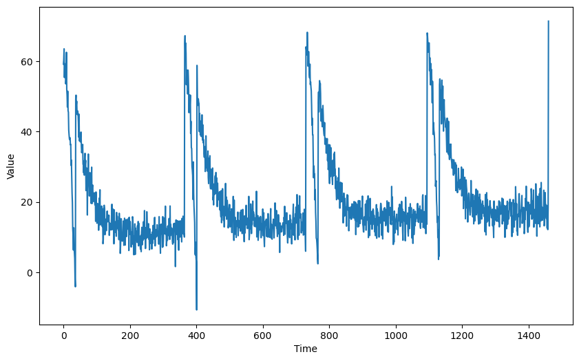
# Plot the generated series
plt.figure(figsize=(10, 6))
plot_series(G.TIME, G.SERIES)
plt.show()
Splitting the data#
def train_val_split(time, series, time_step=G.SPLIT_TIME):

    time_train = time[:time_step]
    series_train = series[:time_step]
    time_valid = time[time_step:]
    series_valid = series[time_step:]

    return time_train, series_train, time_valid, series_valid

time_train, series_train, time_valid, series_valid = train_val_split(G.TIME, G.SERIES)
Processing the data#
def windowed_dataset(series, window_size=G.WINDOW_SIZE, batch_size=G.BATCH_SIZE, shuffle_buffer=G.SHUFFLE_BUFFER_SIZE):

    dataset = tf.data.Dataset.from_tensor_slices(series)
    dataset = dataset.window(window_size + 1, shift=1, drop_remainder=True)
    dataset = dataset.flat_map(lambda window: window.batch(window_size + 1))

    dataset = dataset.shuffle(shuffle_buffer)
    dataset = dataset.map(lambda window: (window[:-1], window[-1]))

    dataset = dataset.batch(batch_size).prefetch(1)

    return dataset
test_dataset = windowed_dataset(series_train, window_size=1, batch_size=5, shuffle_buffer=1)

# Get the first batch of the test dataset
batch_of_features, batch_of_labels = next((iter(test_dataset)))

print(f"batch_of_features has type: {type(batch_of_features)}\n")
print(f"batch_of_labels has type: {type(batch_of_labels)}\n")
print(f"batch_of_features has shape: {batch_of_features.shape}\n")
print(f"batch_of_labels has shape: {batch_of_labels.shape}\n")
print(f"batch_of_features is equal to first five elements in the series: {np.allclose(batch_of_features.numpy().flatten(), series_train[:5])}\n")
print(f"batch_of_labels is equal to first five labels: {np.allclose(batch_of_labels.numpy(), series_train[1:6])}")
batch_of_features has type: <class 'tensorflow.python.framework.ops.EagerTensor'>

batch_of_labels has type: <class 'tensorflow.python.framework.ops.EagerTensor'>

batch_of_features has shape: (5, 1)

batch_of_labels has shape: (5,)

batch_of_features is equal to first five elements in the series: True

batch_of_labels is equal to first five labels: True
Defining the model architecture#
def create_model(window_size=G.WINDOW_SIZE):

    model = tf.keras.models.Sequential([
        tf.keras.layers.Dense(10, activation='relu', input_shape=[window_size]),
        tf.keras.layers.Dense(10, activation='relu'),
        tf.keras.layers.Dense(1)
    ])

    model.compile(loss='mse',
                  optimizer='adam')

    return model
dataset = windowed_dataset(series_train)

model = create_model()

model.fit(dataset, epochs=100)
Evaluating the forecast#
def compute_metrics(true_series, forecast):

    mse = tf.keras.metrics.mean_squared_error(true_series, forecast).numpy()
    mae = tf.keras.metrics.mean_absolute_error(true_series, forecast).numpy()

    return mse, mae
def generate_forecast(series=G.SERIES, split_time=G.SPLIT_TIME, window_size=G.WINDOW_SIZE):
    forecast = []
    for time in range(len(series) - window_size):
        forecast.append(model.predict(series[time:time + window_size][np.newaxis]))

    forecast = forecast[split_time-window_size:]
    results = np.array(forecast)[:, 0, 0]
    return results


# Save the forecast
dnn_forecast = generate_forecast()

# Plot it
plt.figure(figsize=(10, 6))
plot_series(time_valid, series_valid)
plot_series(time_valid, dnn_forecast)
mse, mae = compute_metrics(series_valid, dnn_forecast)

print(f"mse: {mse:.2f}, mae: {mae:.2f} for forecast")
mse: 24.05, mae: 2.99 for forecast