Why do machine learning models lose their predictive power over time?

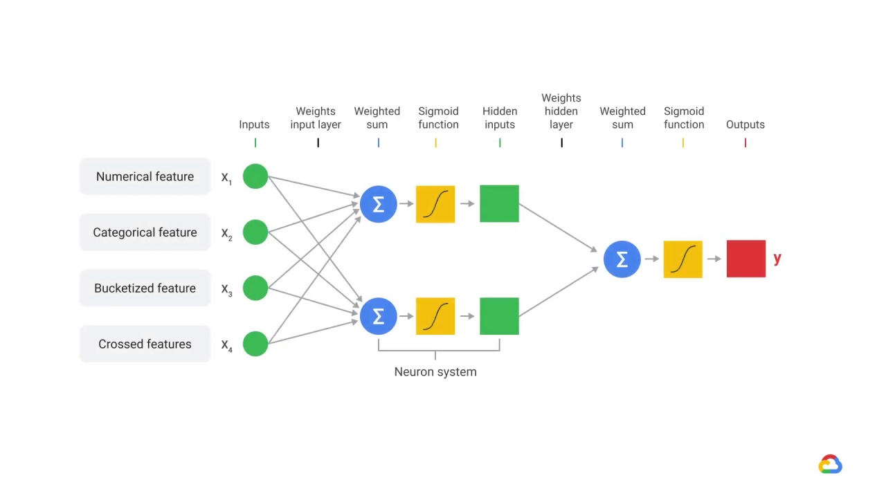
You’ll recall that machine learning models, such as neural networks, accept a feature vector and provide a prediction for our target variable.

These models learn in a supervised fashion where a set of feature vectors with expected output is provided.

The traditional supervised learning assumes that the training and the application data come from the same distribution.

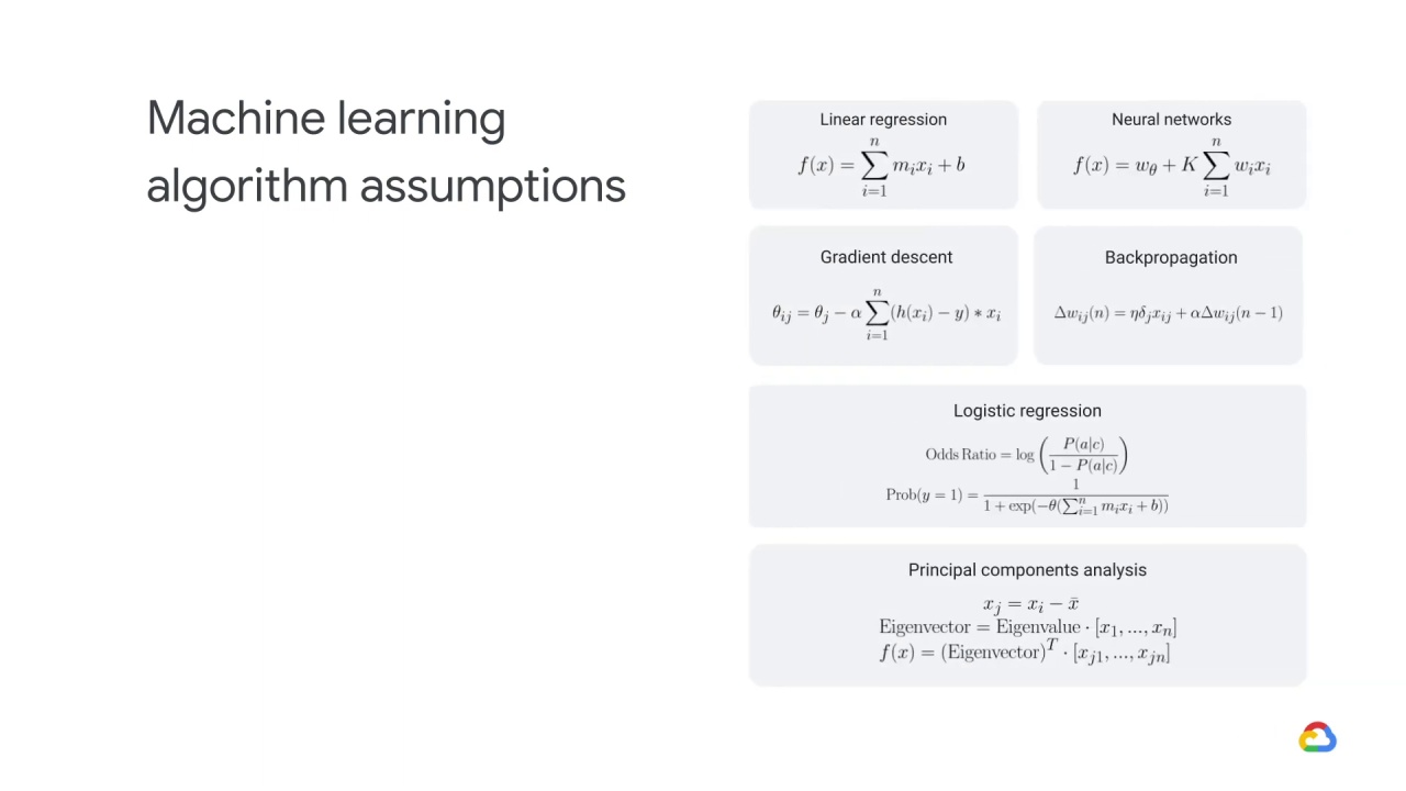
You’ll also remember that traditional machine learning algorithms were developed with certain assumptions.

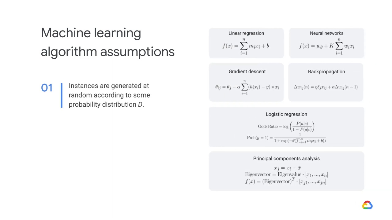
The first is that instances are generated at random according to some probability distribution D.

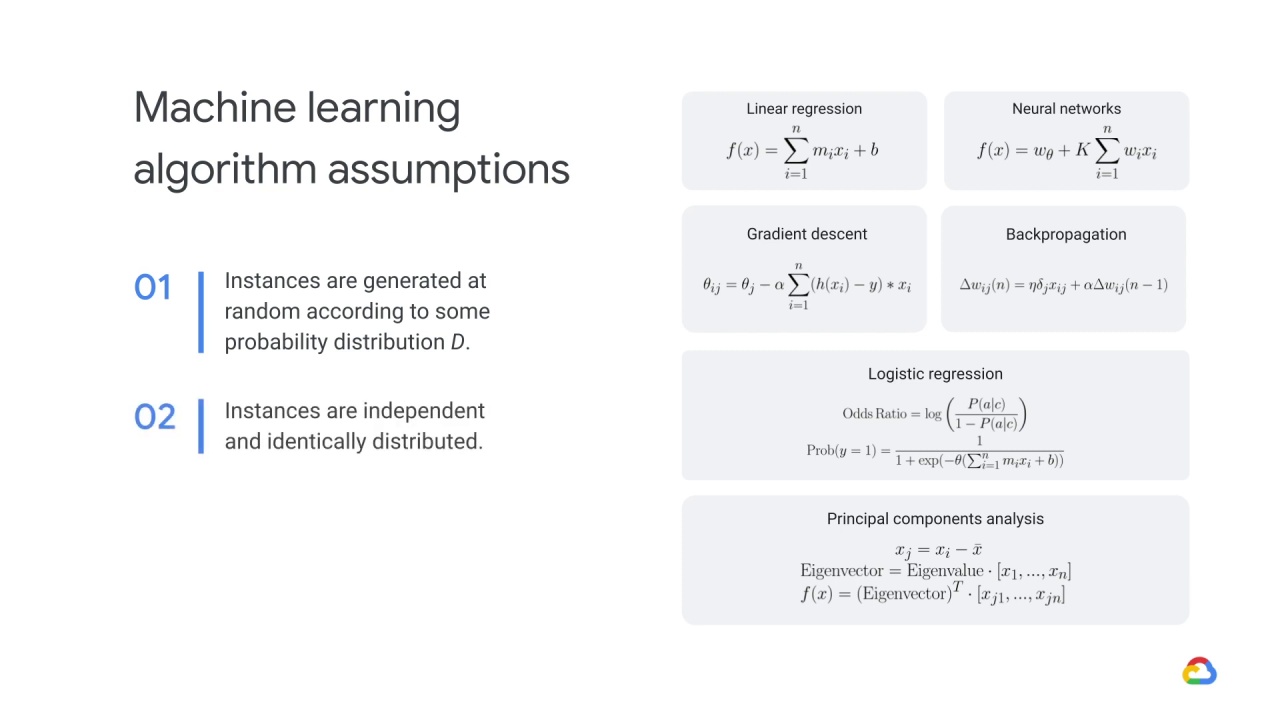
The second is that instances are independent and identically distributed.

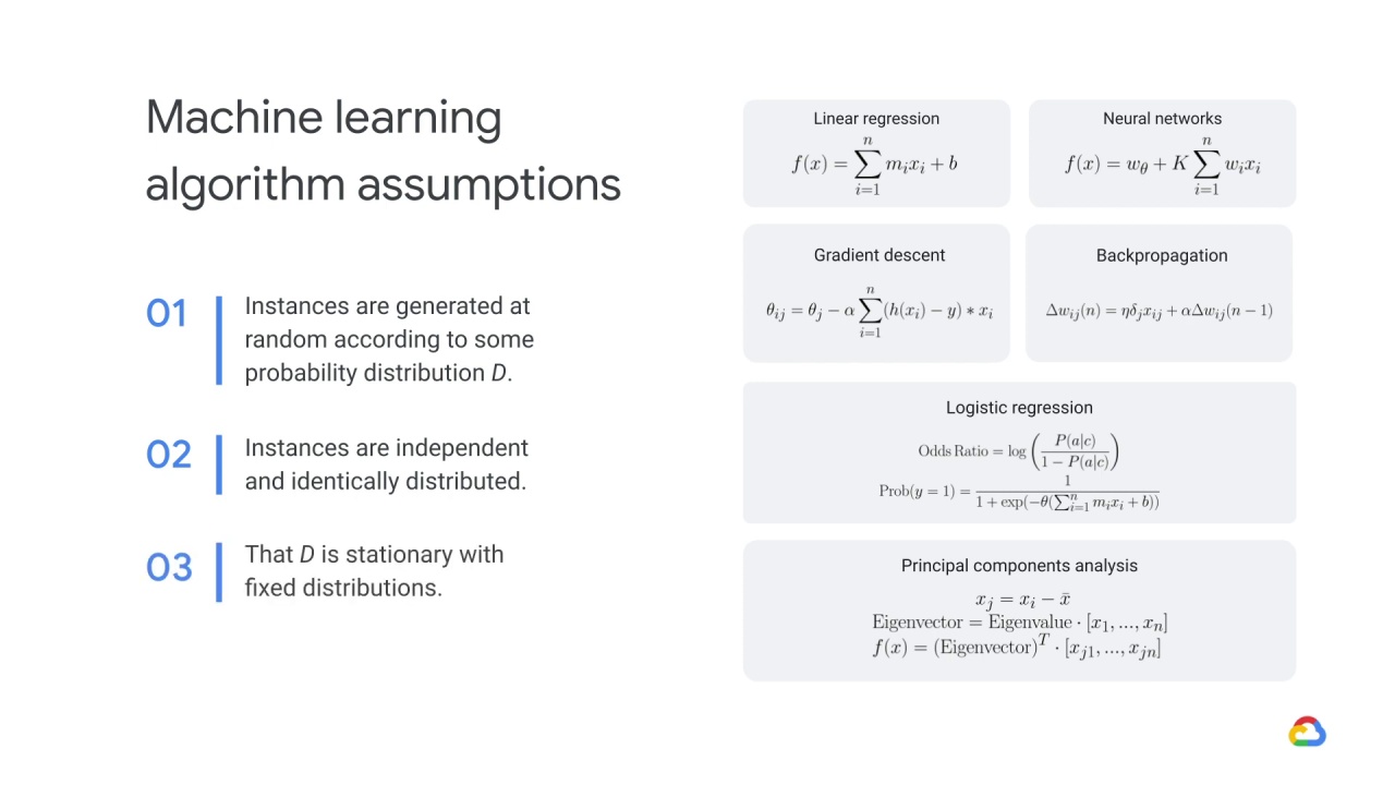
And the third assumption is that D is stationary with fixed distributions.

Drift is the change in an entity with respect to a baseline.

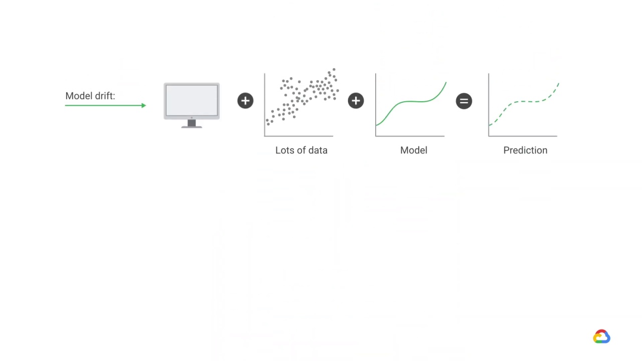
In the case of production ML models, this is the change between the real-time production data and a baseline data set, likely the training set, that is representative of the task the model is intended to perform.

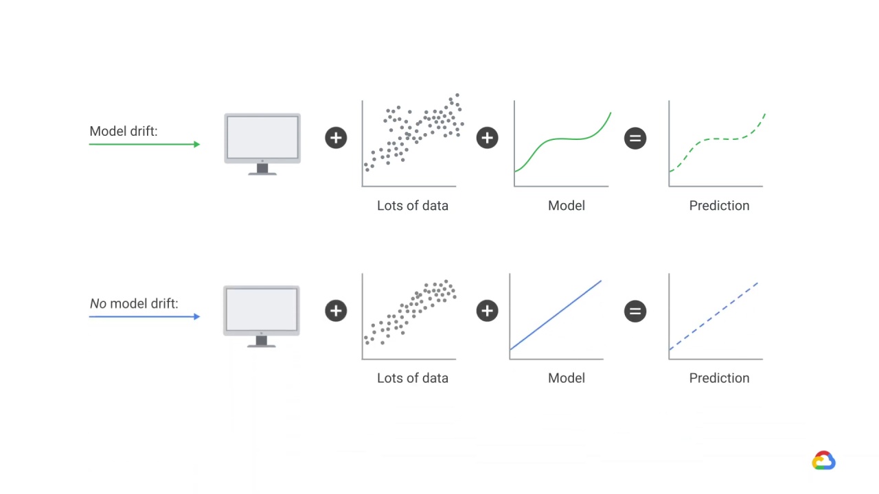
If your model were running in a static environment, using static or stationary data - for example data whose statistical properties do not change, then model drift wouldn’t occur and your model would not lose any of its predictive power because the data you’re predicting comes from the same distribution as the data used for training.

But production data can diverge or drift from the baseline data over time due to changes in the real world.

There are several types of drift in ML models…

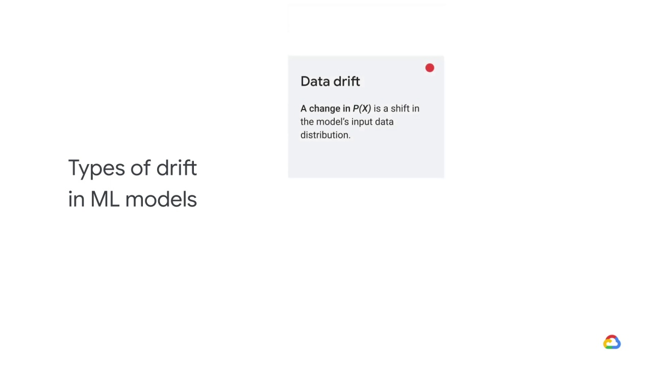
Data Drift or change in probability of X, \(P(X)\), is a shift in the model’s input data distribution.

For example, incomes of all applicants increase by 5%, but the economic fundamentals are the same.

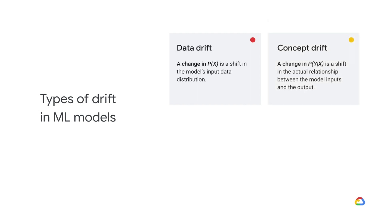
Concept drift or change in probability of Y given X, \(P(Y|X)\), is a shift in the actual relationship between the model inputs and the output.

An example of concept drift is when macroeconomic factors make lending riskier, and there is a higher standard to be eligible for a loan.

In this case, an income level that was earlier considered creditworthy is no longer creditworthy.

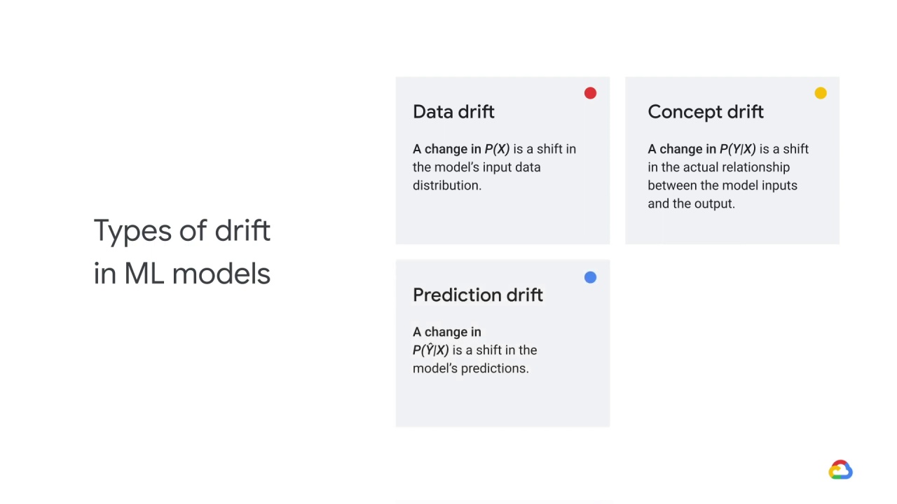
Prediction drift or change in the predicted value of Y given X, \(P(\hat{Y}|X)\) is a shift in the model’s predictions.

For example, a larger proportion of credit-worthy applications when your product was launched in a more affluent area.

Your model still holds, but your business may be unprepared for this scenario.

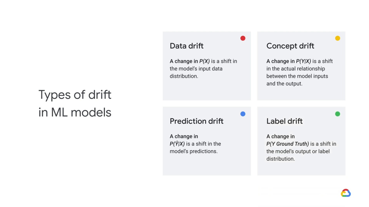
Label drift or change in the predicted value of Y as your target variable \(P(Y\) Ground Truth\()\) is a shift in the model’s output or label distribution.

Data drift,

feature drift,

population,

and covariate shift

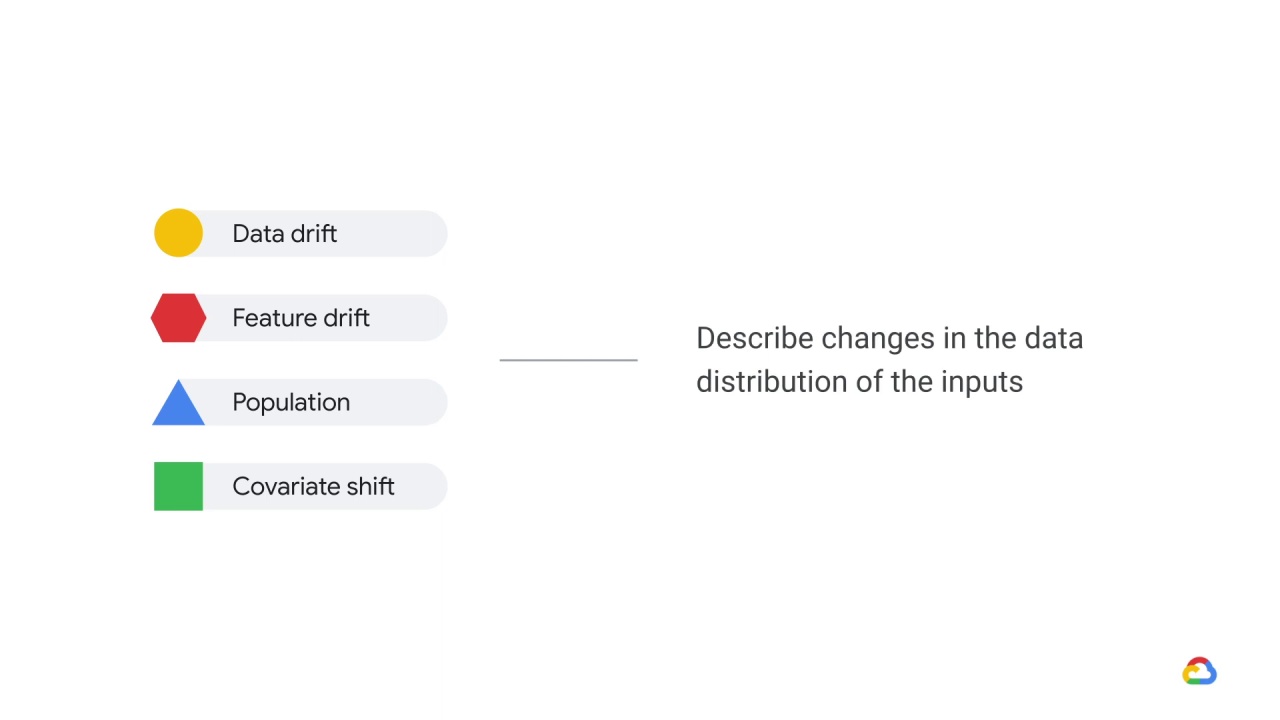
are all names to describe changes in the data distribution of the inputs.

When data shift occurs, or when you observe that the model performs worse on unknown data regions, that means that the input data has changed.

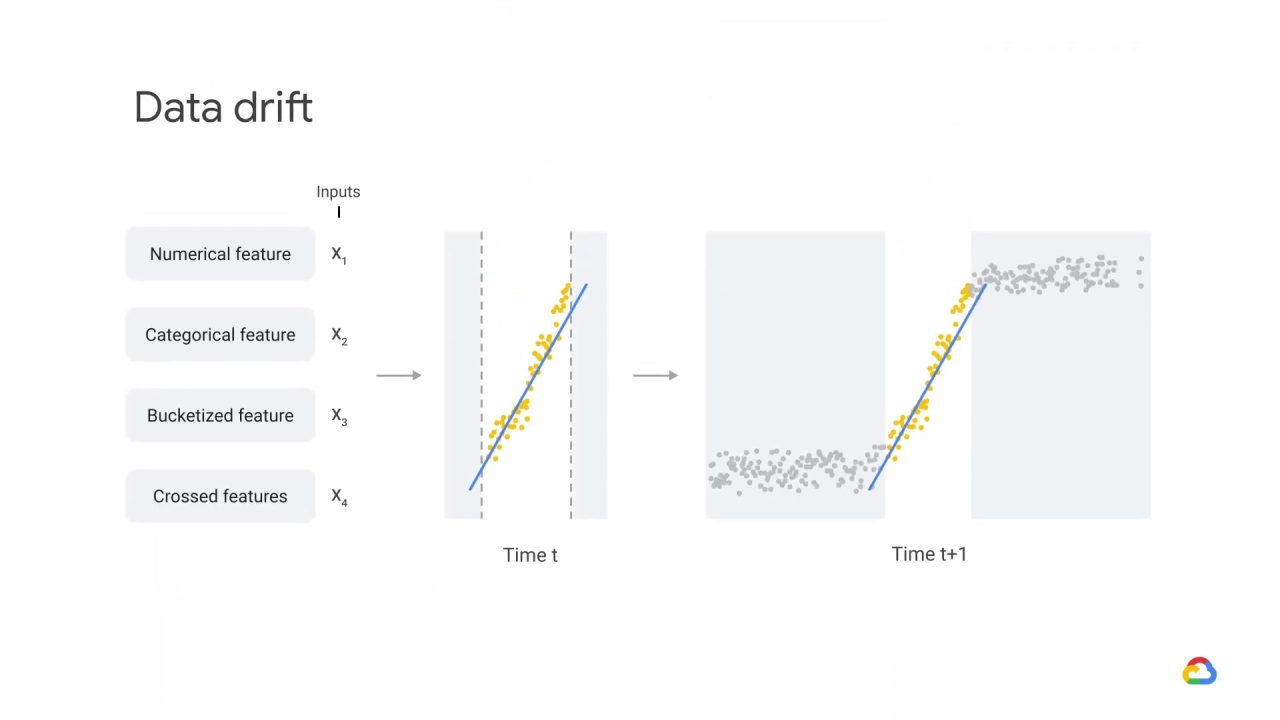
The distribution of the variables is meaningfully different.

As a result, the trained model is not relevant for this new data.

It would still perform well on the data that is similar to the “old” one!

The model is fine on the “old data”, but in practical terms, it became dramatically less useful since we are now dealing with a new feature space.

Indeed, the relationships between the model inputs and outputs have changed.

In contrast, concept drift occurs when there is a change in the relationship between the input feature and the label (or target).

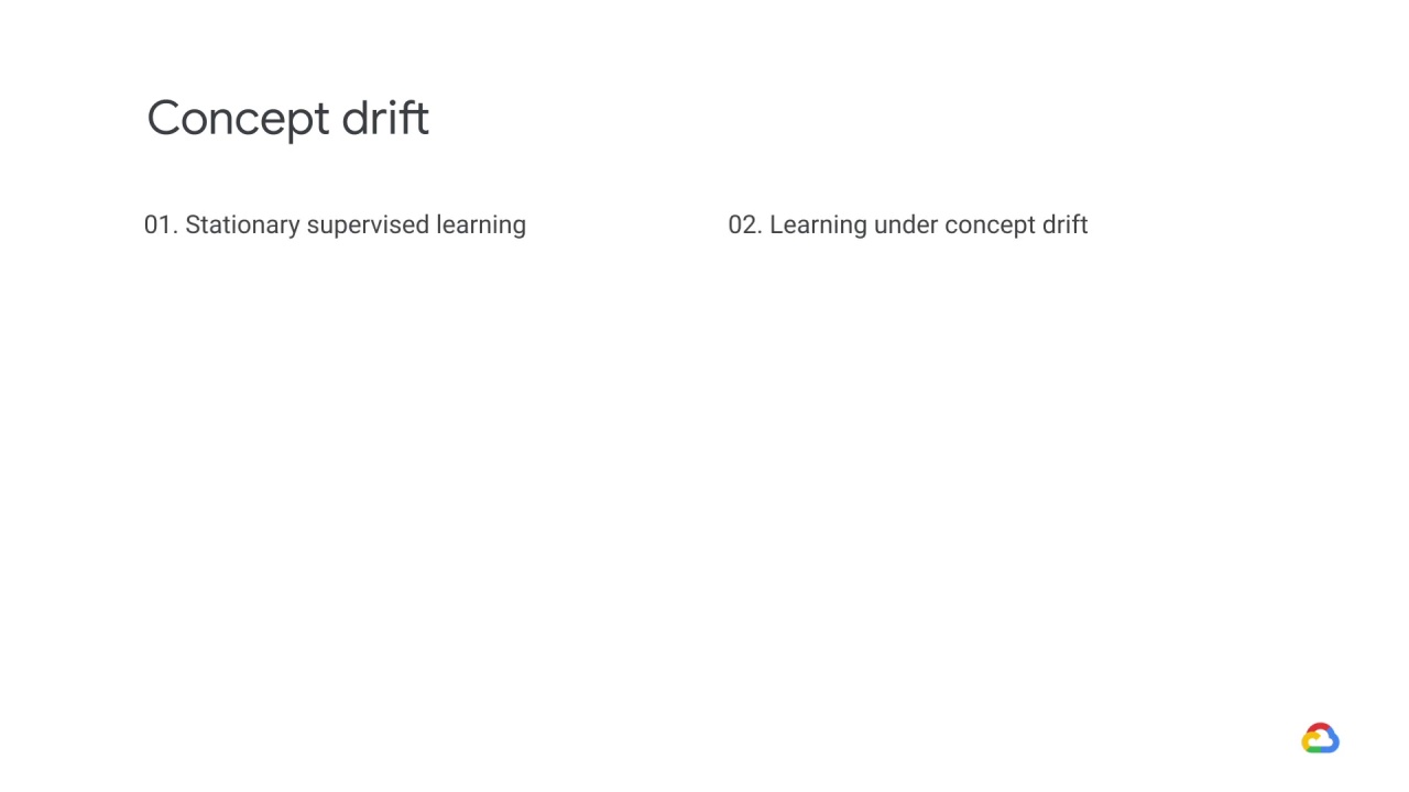
Let’s explore two examples of concept drift which highlight the change in the relationship between the input feature and the label.

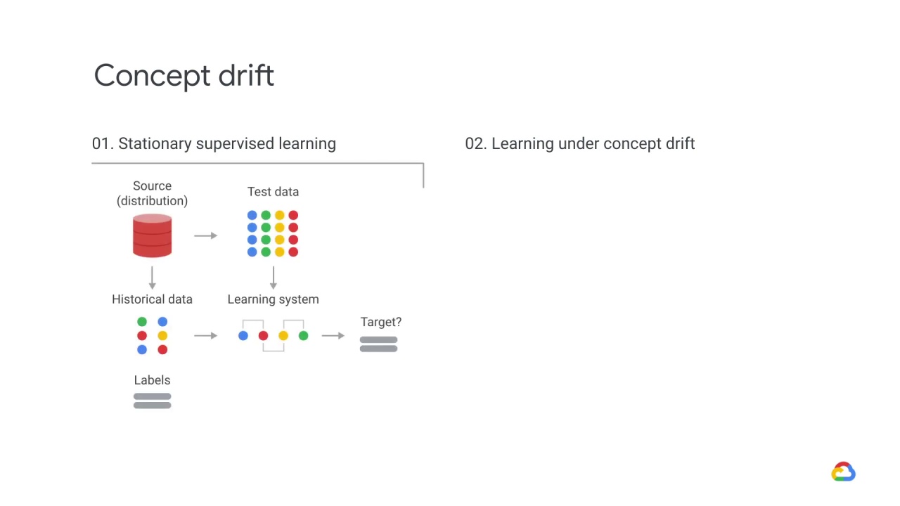
In this first example, stationary supervised learning, historical data is used to make predictions.

You might recall that in supervised learning, a model is trained from historical data and that data is used to make predictions.

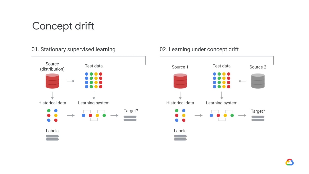
This second example is supervised learning under concept drift, where a new, secondary data source is ingested to provide both historical data and new data to make predictions.

This new data could be in batch or real time.

Whatever the form, it’s important to know that the statistical properties of the target variable may change over time.

As a result, an interpretation of the data changes with time, while the general distribution of the feature input may not.

This illustrates concept drift, where the statistical properties of the class variable (the target we want to predict) changes over time.

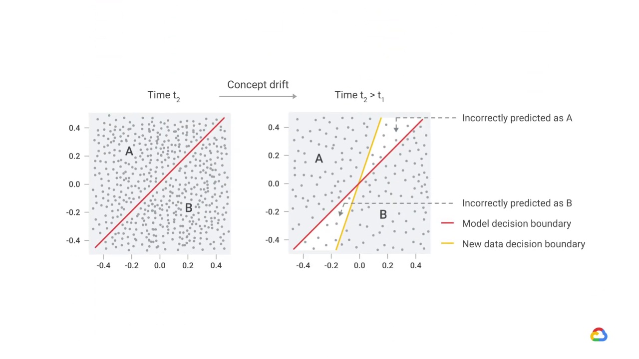
In this supervised learning classification example, when the distribution of the label changes, it could mean that the relationship between features and labels is changing as well.

At the very least, it’s likely that our model’s predictions, which will typically match the distribution of the labels on the data on which it was trained, will be significantly less accurate.

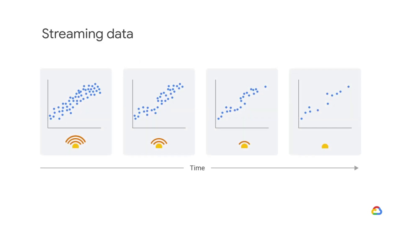
Let’s take a look at one other example.

This one deals with streaming data.

Data flows continuously over time in dynamic environments - particularly for streaming data, such as e-commerce, user modeling, spam emails, fraud detection, and intrusion, Changes in underlying data occur due to changing personal interests, changes in population, or adversary activities, or they can be attributed to a complex nature of the environment.

In this example, a sensor’s measurement can drift due to a fault with the sensor or aging, changes in operation conditions or control command, and machine degradation as a result of wearing.

In these cases, the distribution of the feature inputs and the labels or targets may change - which will impact model performance and lead to model drift.

There is no guarantee that future data will follow similar distributions of past data in a stream setting.

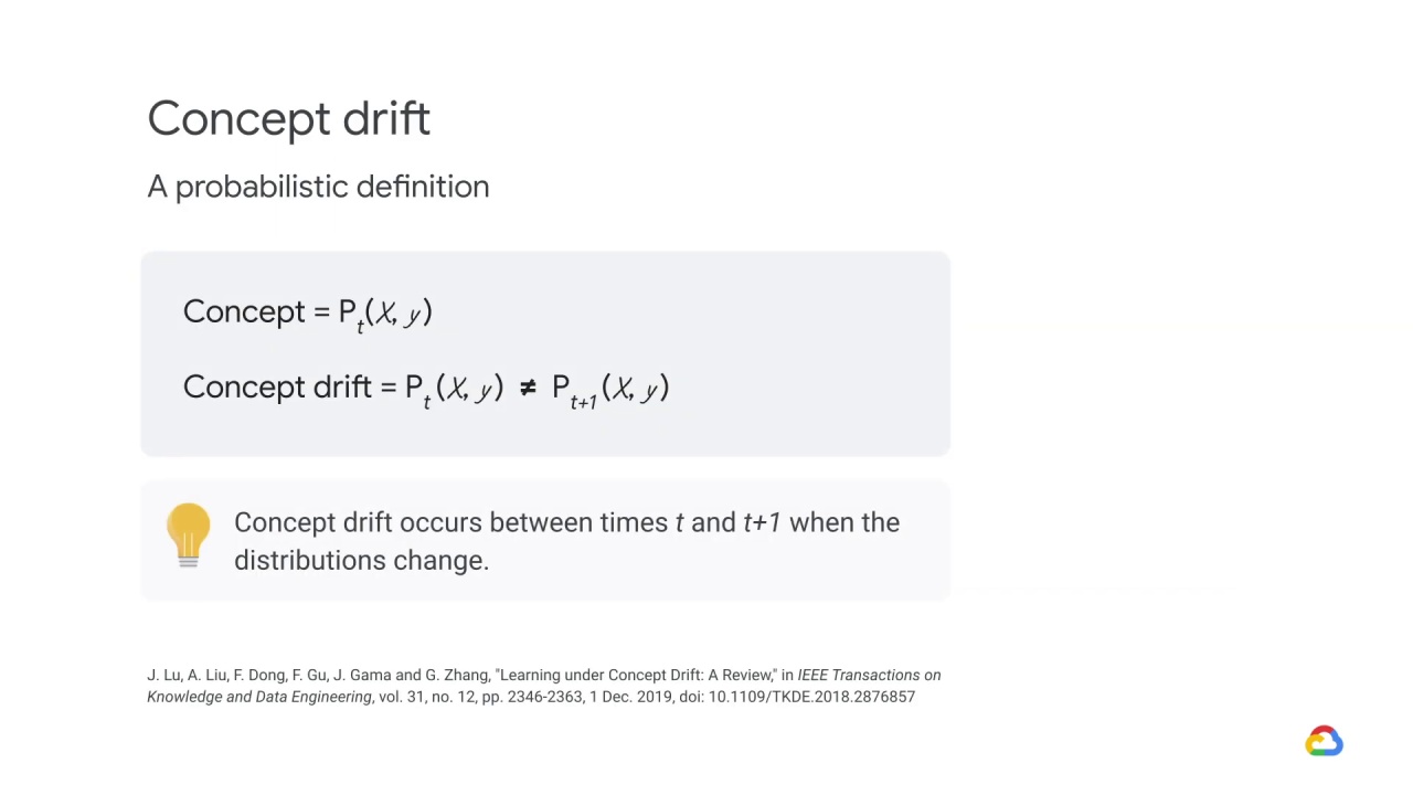
Accordingly, concept drift at time \(t\) can be defined as the change of joint probability of \(X\) and \(y\) at time \(t\).

The joint probability \(P_t(X, y)\) can be decomposed into two parts as the probability of \(X\) times the probability of \(y\) given \(X\).

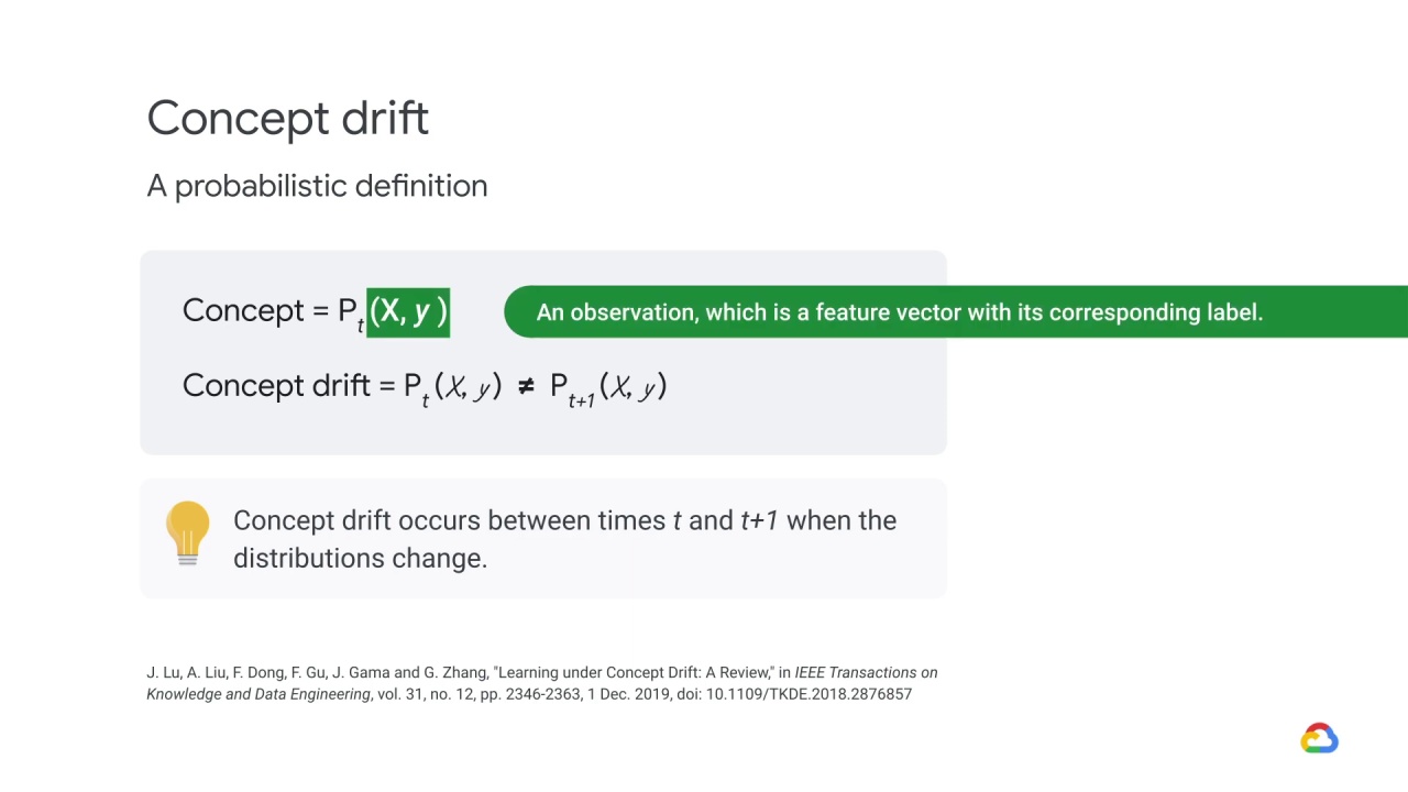
Let’s be a little more careful here with the definition of concept drift.

Let’s use \(X\) to a feature vector and y to its corresponding label.

Of course, when doing supervised learning, our goal is to understand the relationship between X and y.

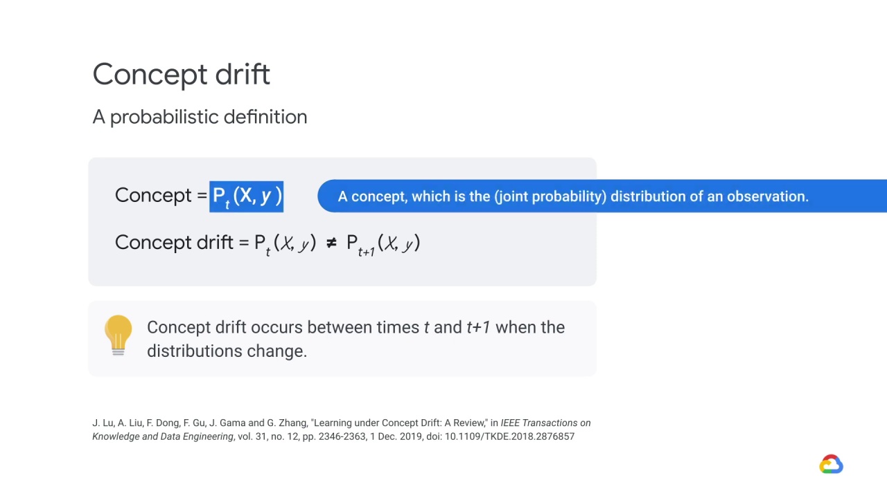
We will define a concept as a description of the distribution of our observations.

More precisely, you can think of this as a joint probability distribution of our observations.

However, this concept could depend on time! Otherwise concept drift would be a non-issue, right?

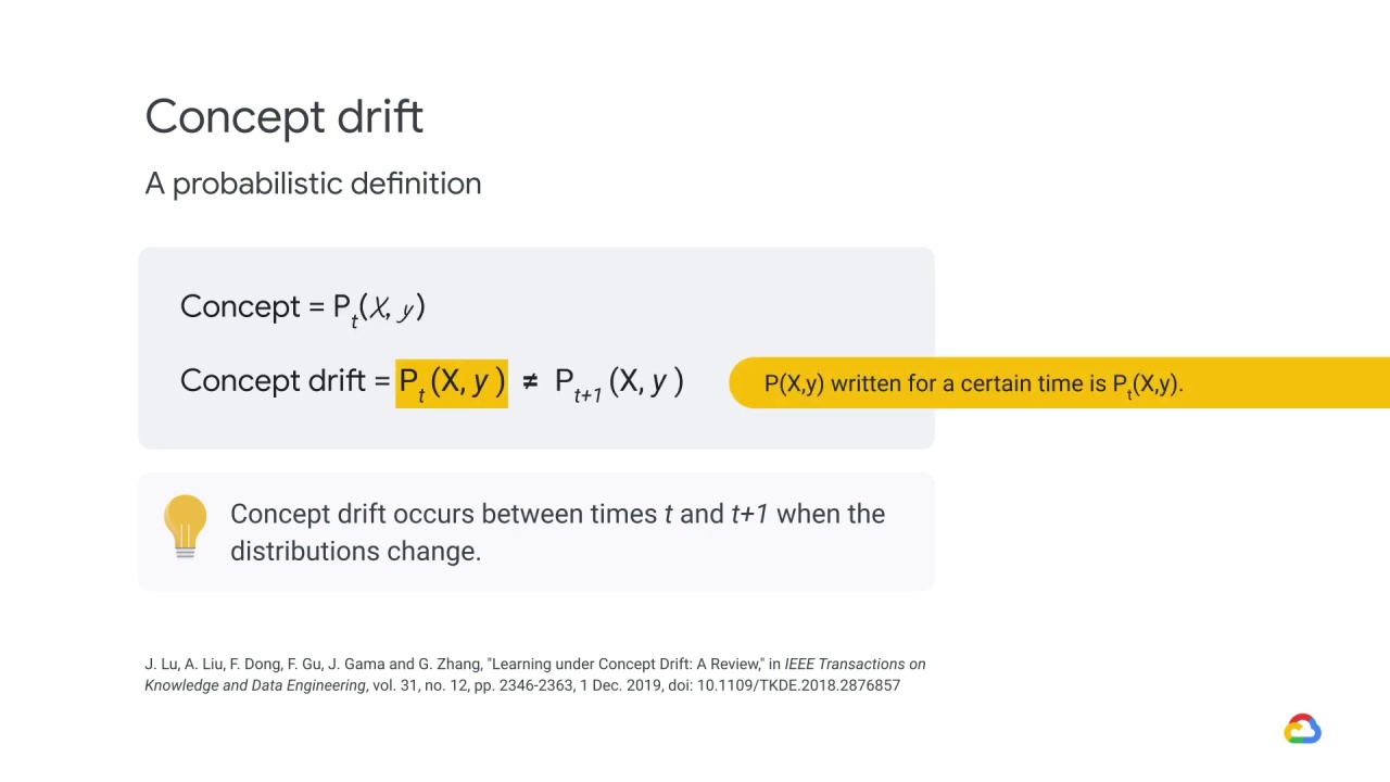
We’ll use the notation probability of \(X\) and \(y\) at time \(t\) \(P_t(X,y)\) when we want to consider the probability of \(X\) and \(y\) \(P(X,y)\) at a specific time.

Now it’s easy to give a more rigorous description of concept drift.

Simply put,

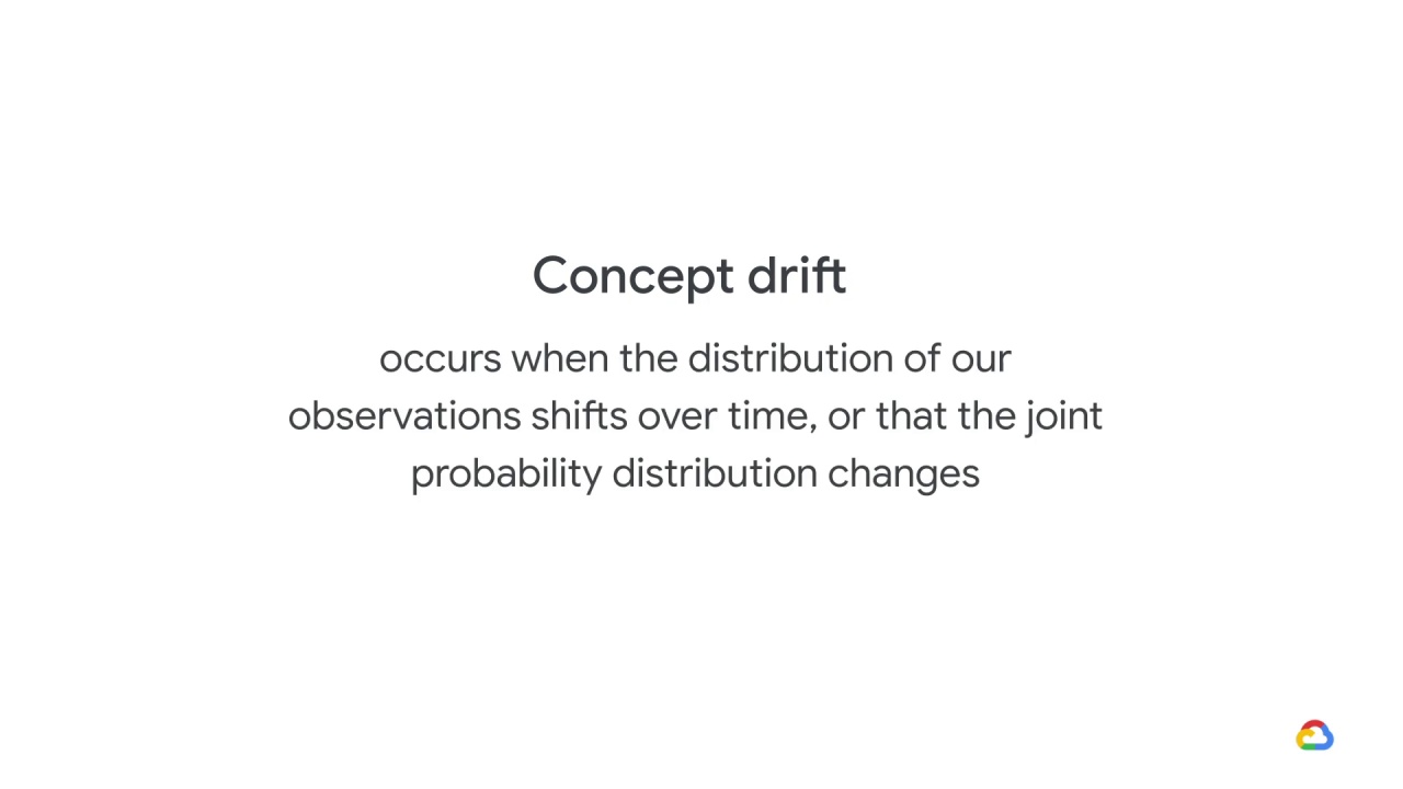
concept drift occurs when the distribution of our observations shifts over time, or that the joint probability distribution we mentioned before changes.

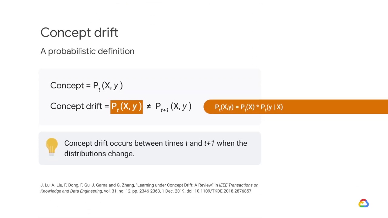
We can break down this distribution into two parts using properties of joint distributions.

• First we have the distribution of the feature space, probability of \(X\) \(P(X)\), and then what we can think of as a description of our decision boundary, the probability of \(y\) given \(X\) \(P(y | X)\).

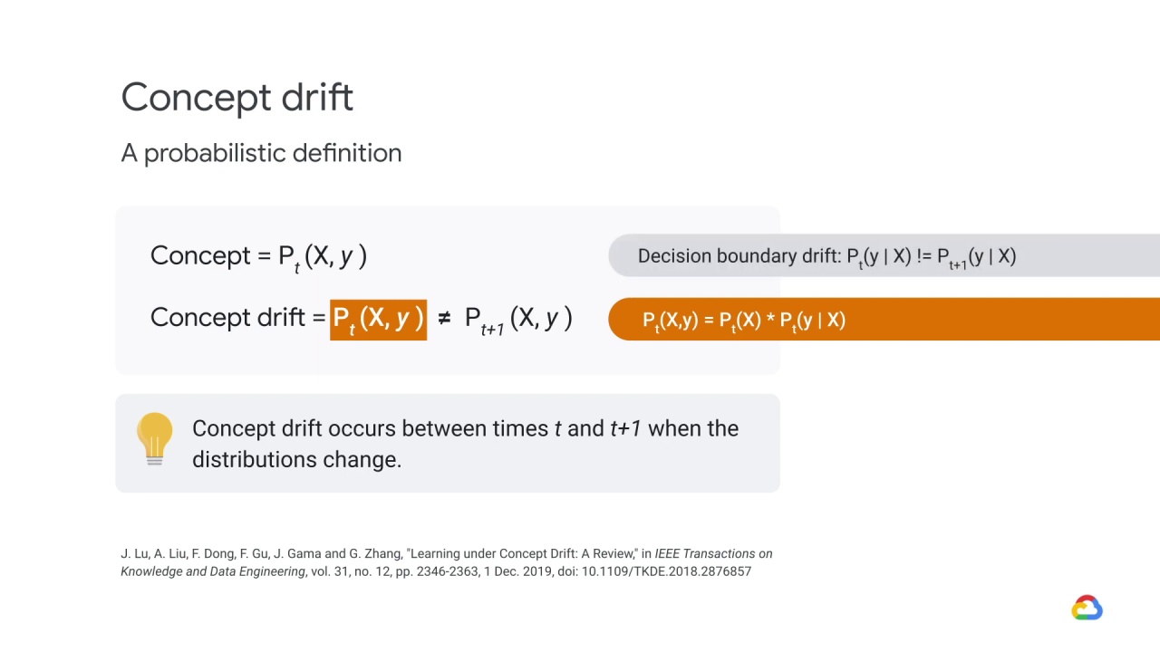
• If the drift is occurring for the decision boundary, then we call this decision boundary drift.

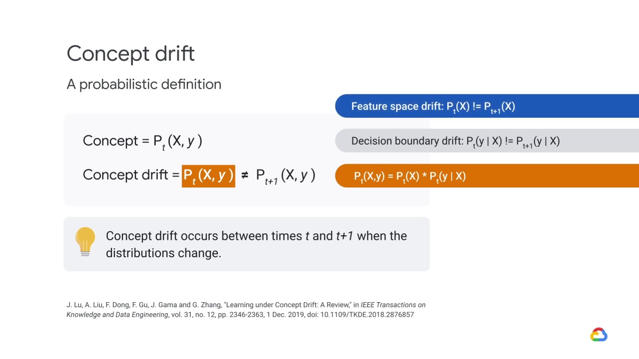
• Likewise, if the drift is occurring for the feature space, we call this feature space drift.

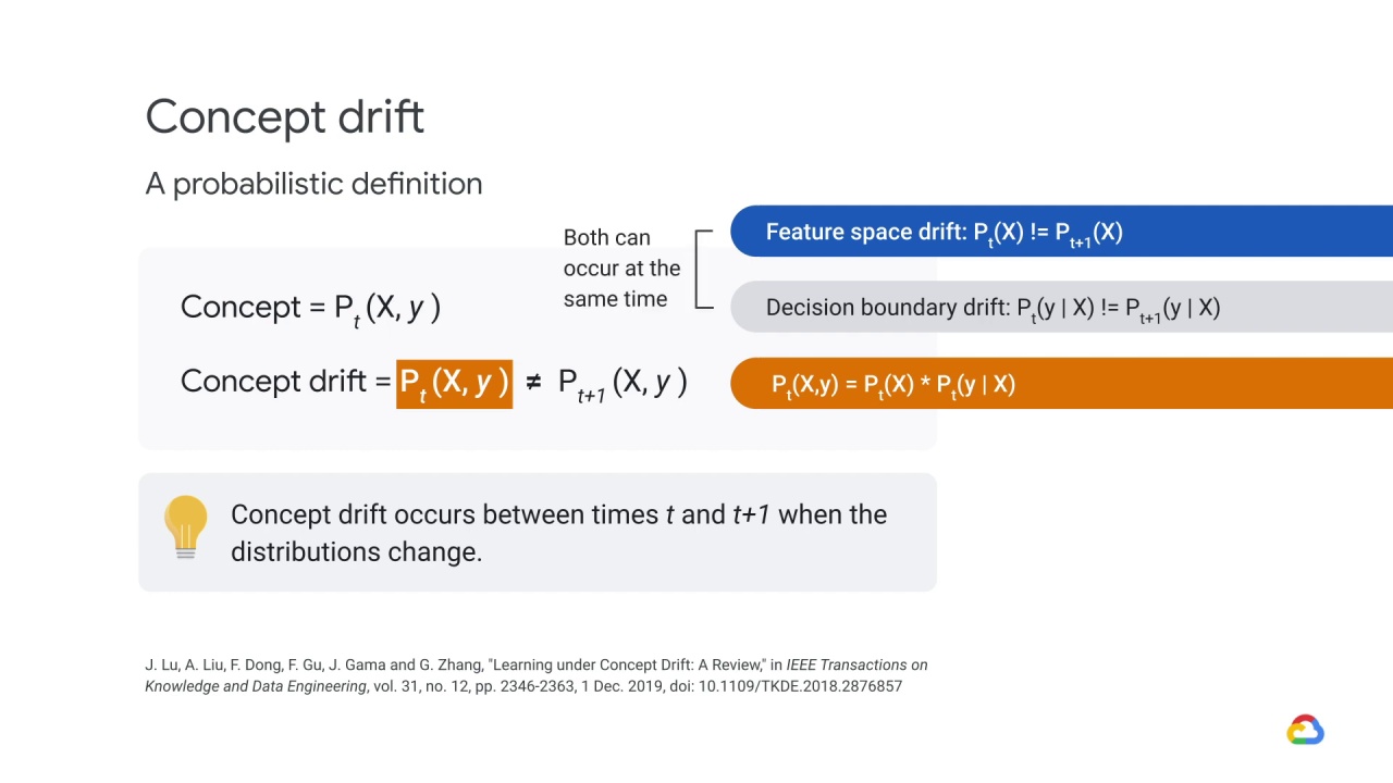
• Of course, both can be happening at the same time, and this can make it complicated to understand where the changes are happening!

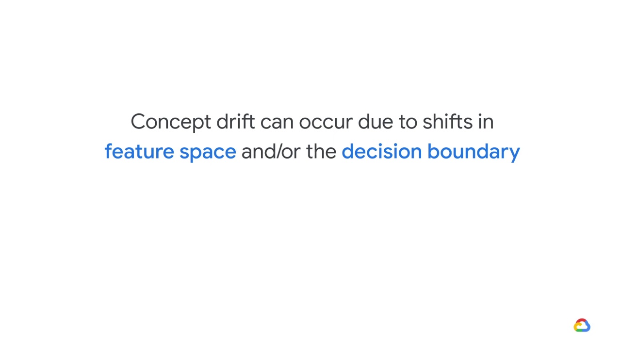
Concept drift can occur due to shifts in the feature space and/or the decision boundary

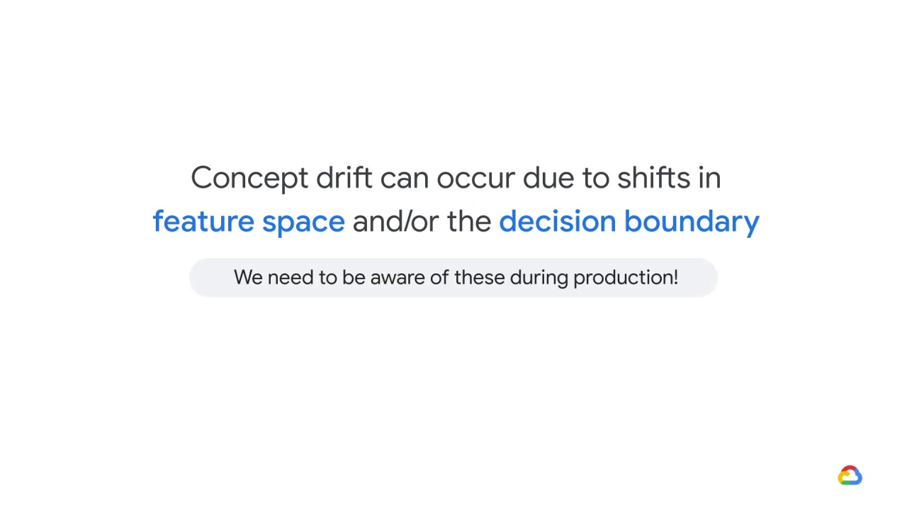
so we need to be aware of these during production.

If the data is changing, or if the relationship between the features and the label is changing, this is going to cause issues with our model.

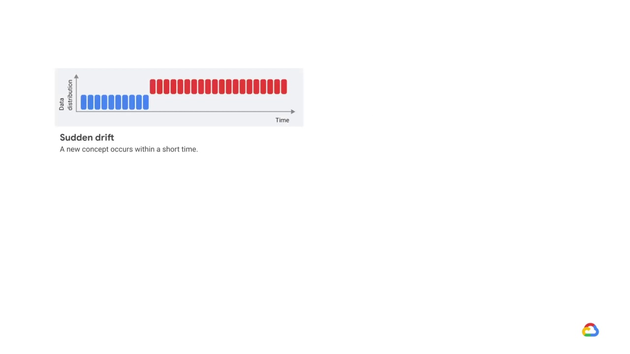
There are different types of concept drift.

• In sudden drift a new concept occurs within a short time.

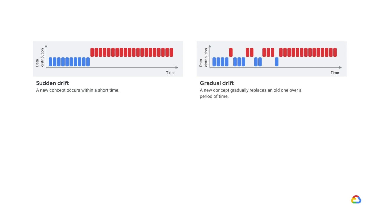
In gradual drift a new concept gradually replaces an old one over a period of time.

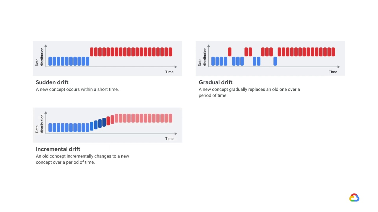
In incremental drift an old concept incrementally changes to a new concept over a period of time.

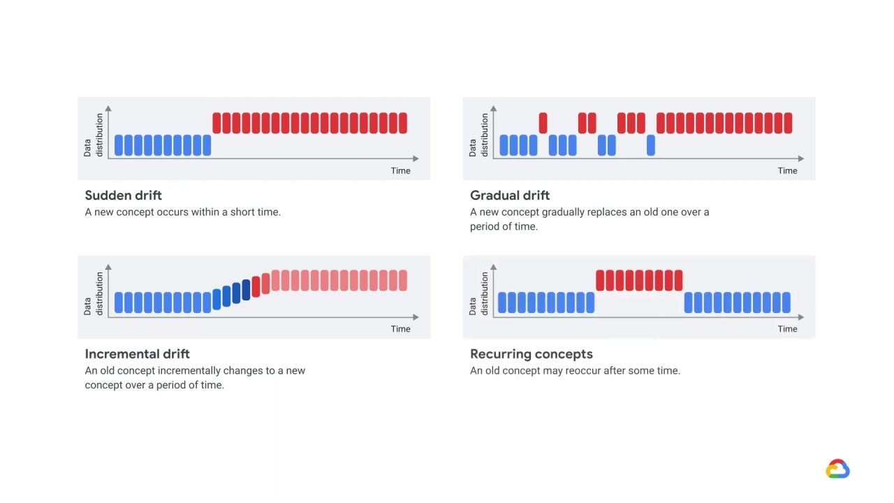
And in recurring concepts an old concept may reoccur after some time