The mirrored strategy is the simplest way to get started with distributed training.

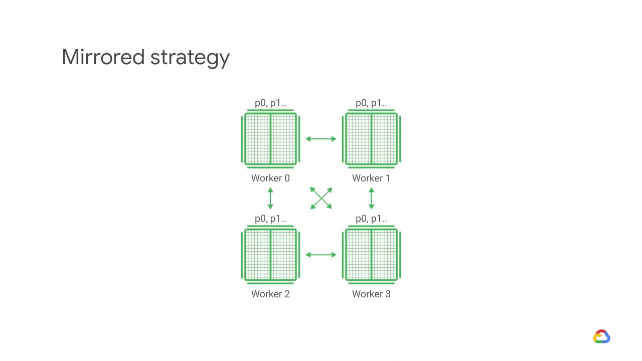
It is a single machine with multiple GPU devices that creates one replica of the model on each GPU device.

During training, one mini-batch is split into N parts, where N equals the number of GPUS, and each part feeds to one GPU device.

For this setup, the TensorFlow mirrored strategy manages the coordination of data distribution and gradient updates across all of the GPUs.

Let’s look at an image classification example where a Keras ResNet model with the functional API is defined.

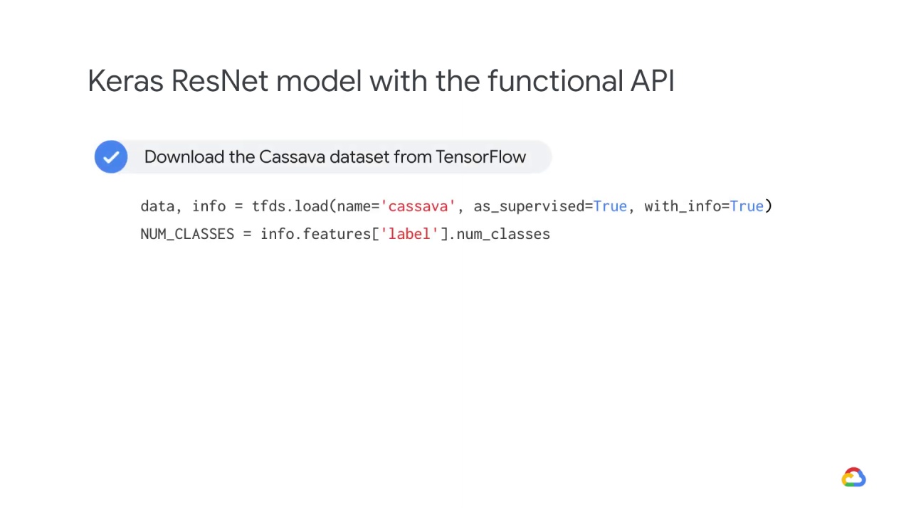
First, download the Cassava dataset from TensorFlow Datasets.

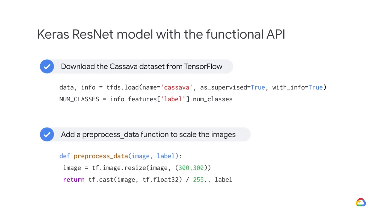
Then, add a preprocess_data function to scale the images.

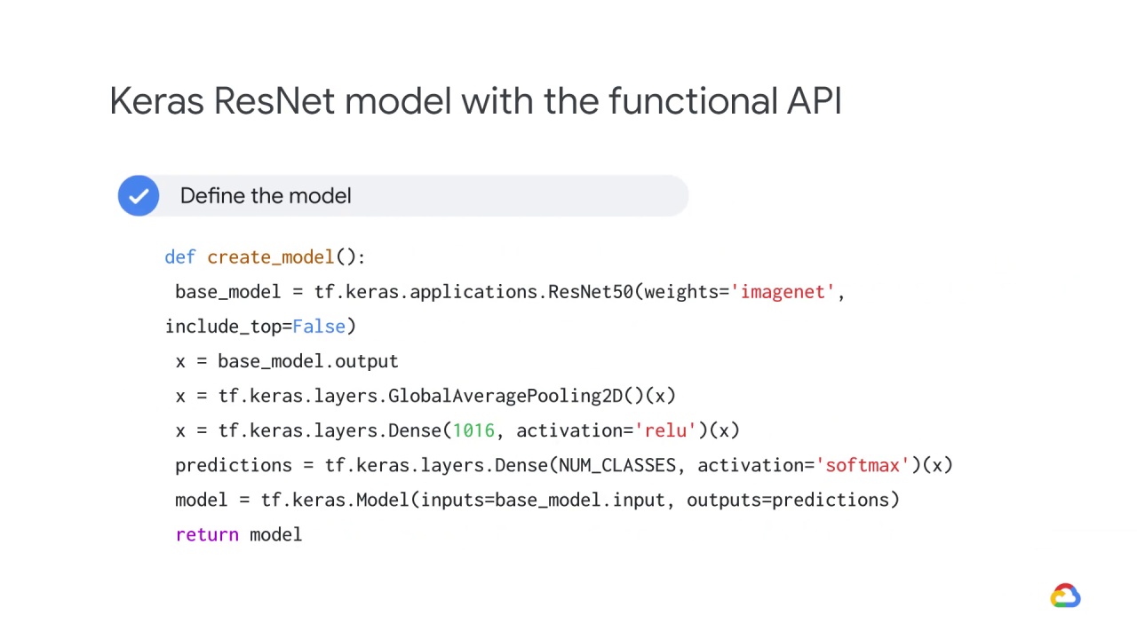
Then, define the model.

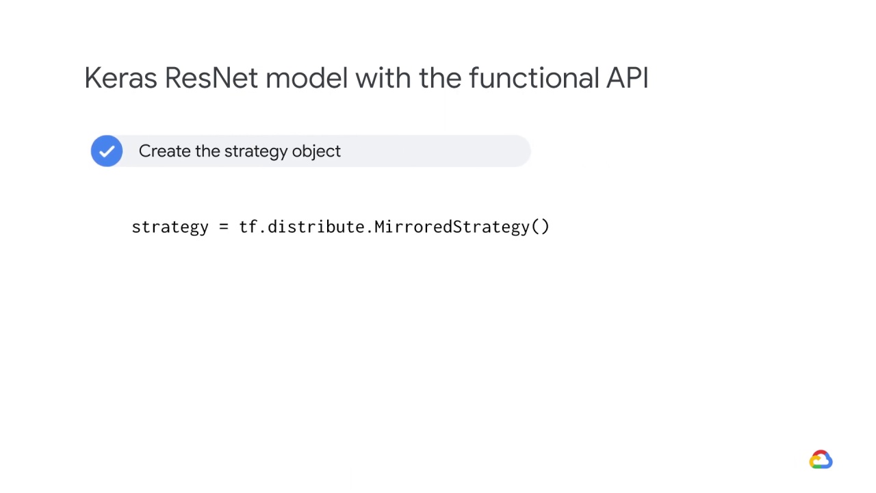
Let’s create the strategy object using tf.distribute.MIrroredStrategy.

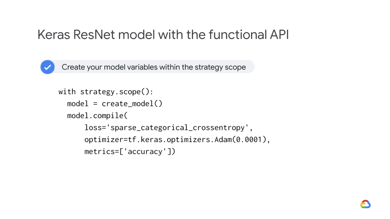
Next, let’s create the model with variables within the strategy scope.

These variables include the model, spare_categorical_crossentropy for loss, a Keras optimizer, and metrics variables to compute accuracy.

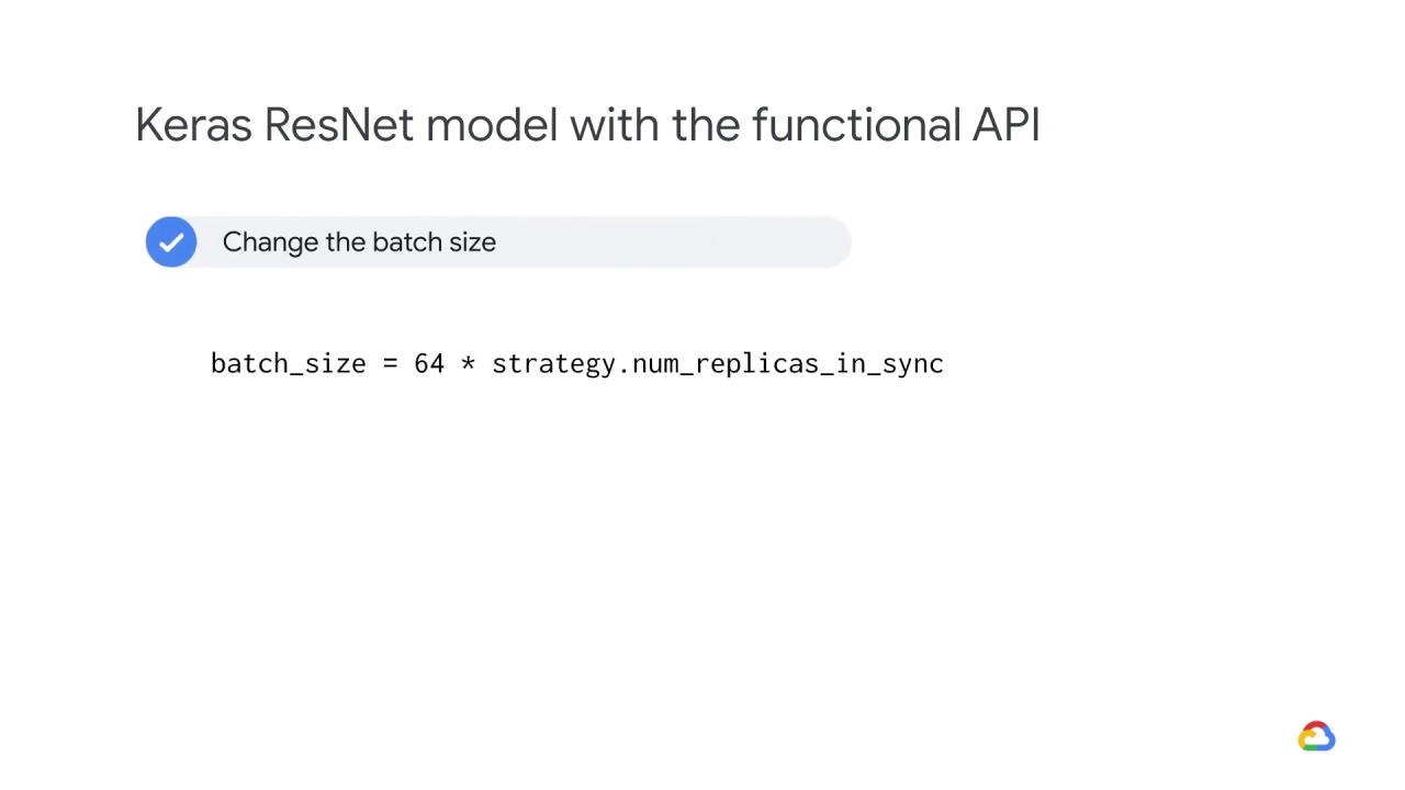
The last change you will want to make is to the batch size.

When you carry out distributed training with the tf.distribute.Strategy API and tf.data, the batch size now refers to the global batch size.

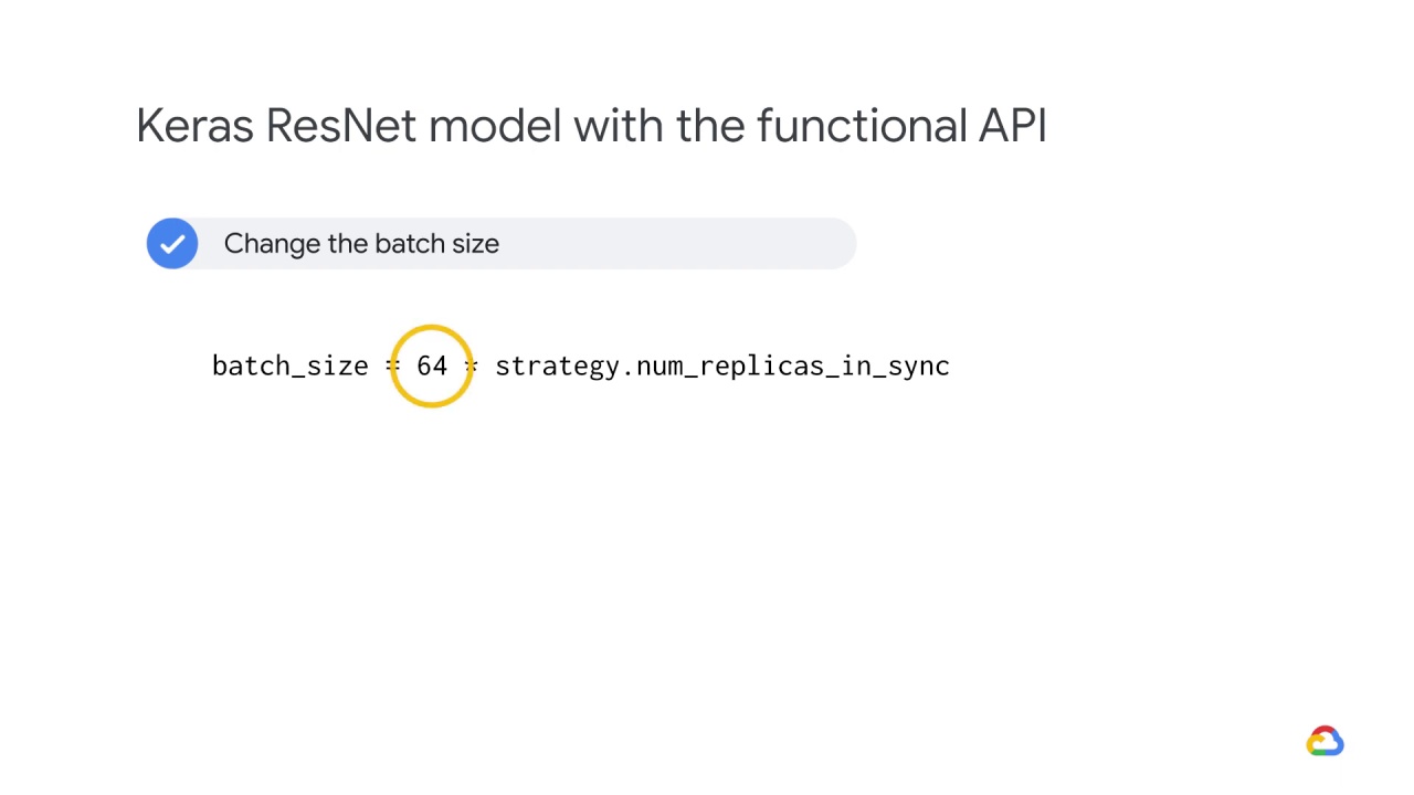
In other words, if you pass a batch size of 64, and you have two GPUs, then each machine will process 32 examples per step.

In this case, 64 is known as the global batch size, and 32 as the per replica batch size.

To make the most out of your GPUs, you will want to scale the batch size by the number of replicas, which is two in this case because there is one replica on each GPU.

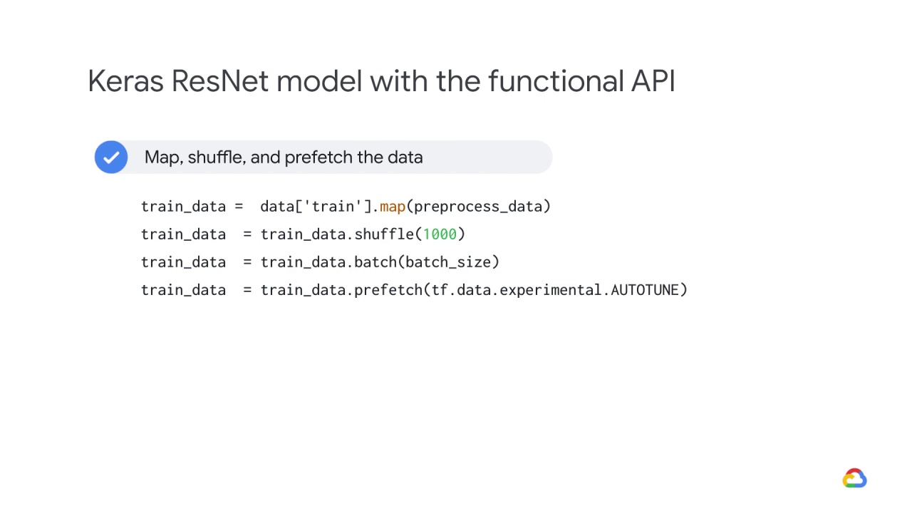
From there, map, shuffle, and prefetch the data.

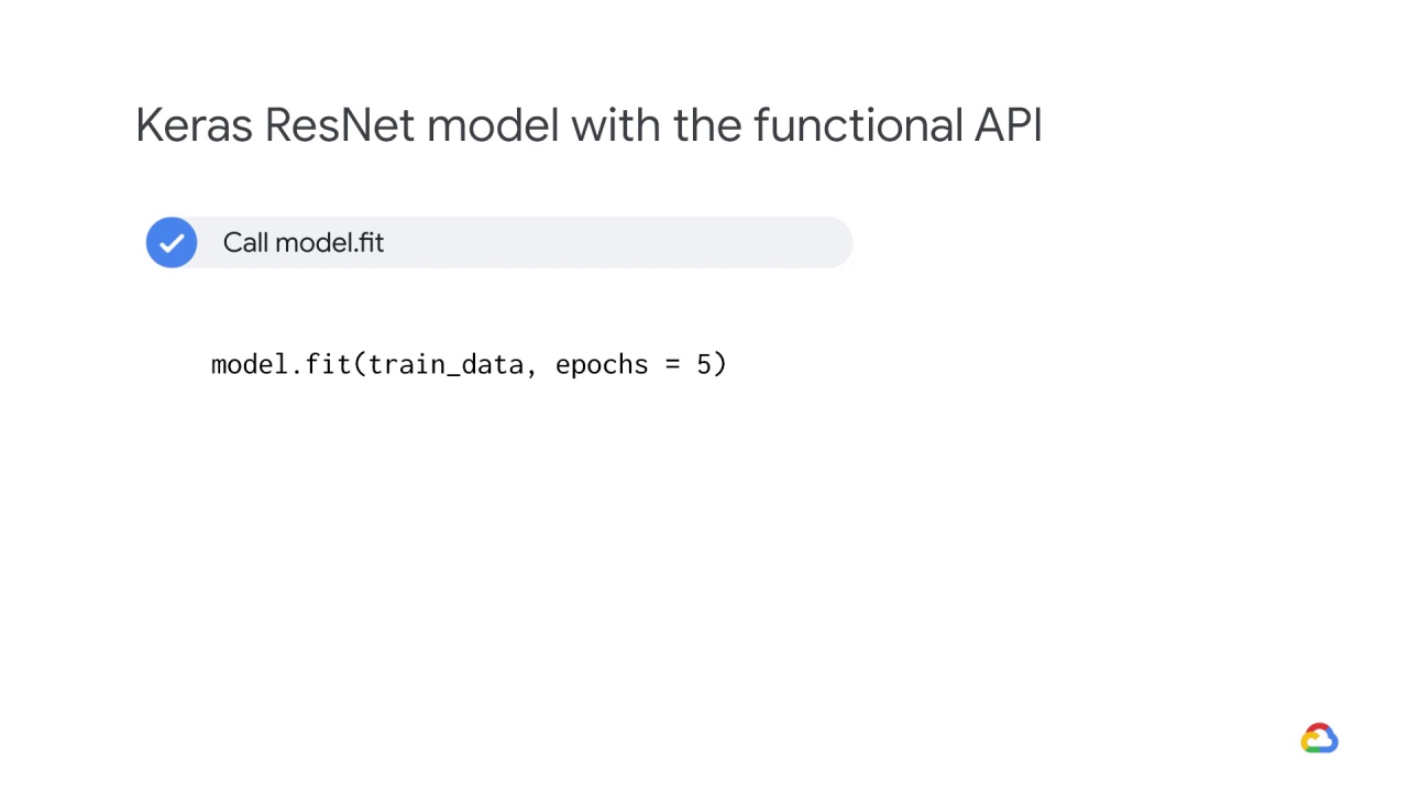
You then call model.fit on the training data.

Here we are going to run five passes of the entire training dataset.

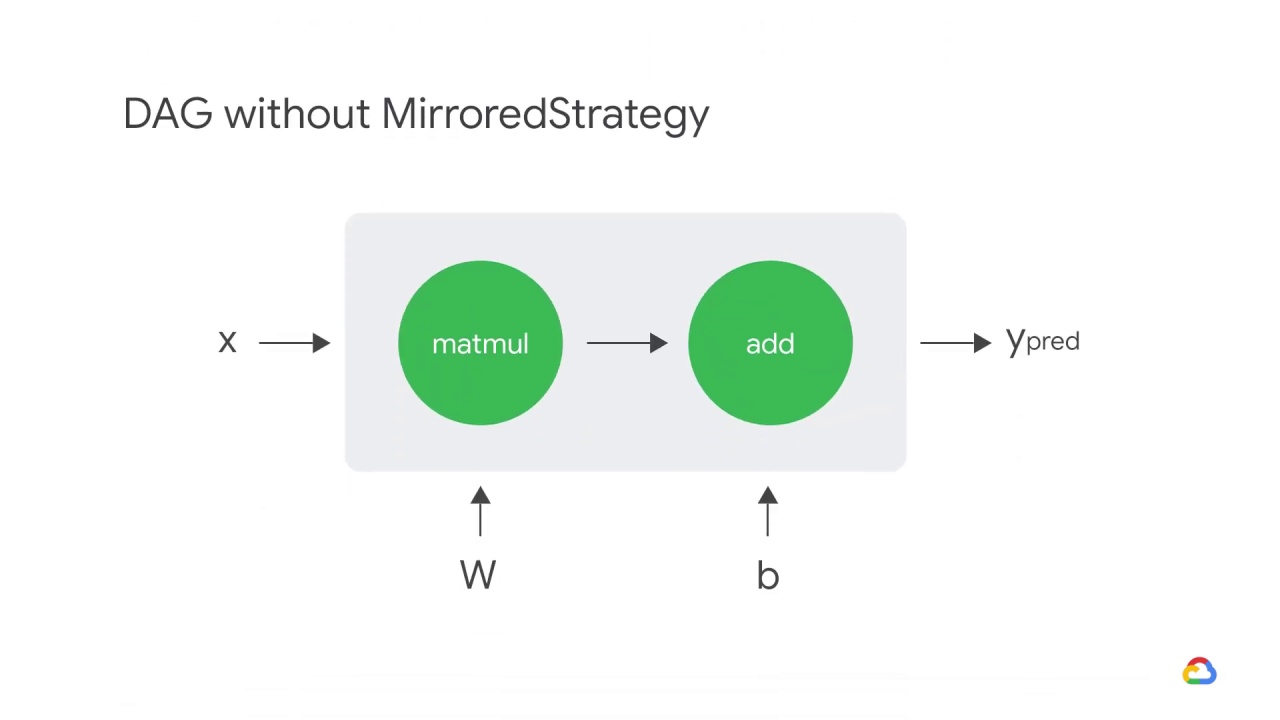
Let’s take a brief look at what actually happens when we call model.fit before adding a strategy.

For simplicity, imagine you have a simple linear model instead of the ResNet50 architecture.

In TensorFlow, you can think of this simple model in terms of its computational graph (or Directed Acyclic Graph - or DAG).

Here, the matmul op takes in the X and W tensors, which are the training batch and weights respectively.

The resulting tensor is then passed to the add op with the tensor b, which is the model’s bias terms.

The result of this op is ypred, which is the model’s predictions.

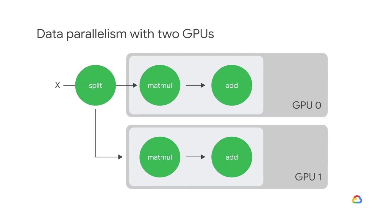
Here is an example of data parallelism with two GPUs.

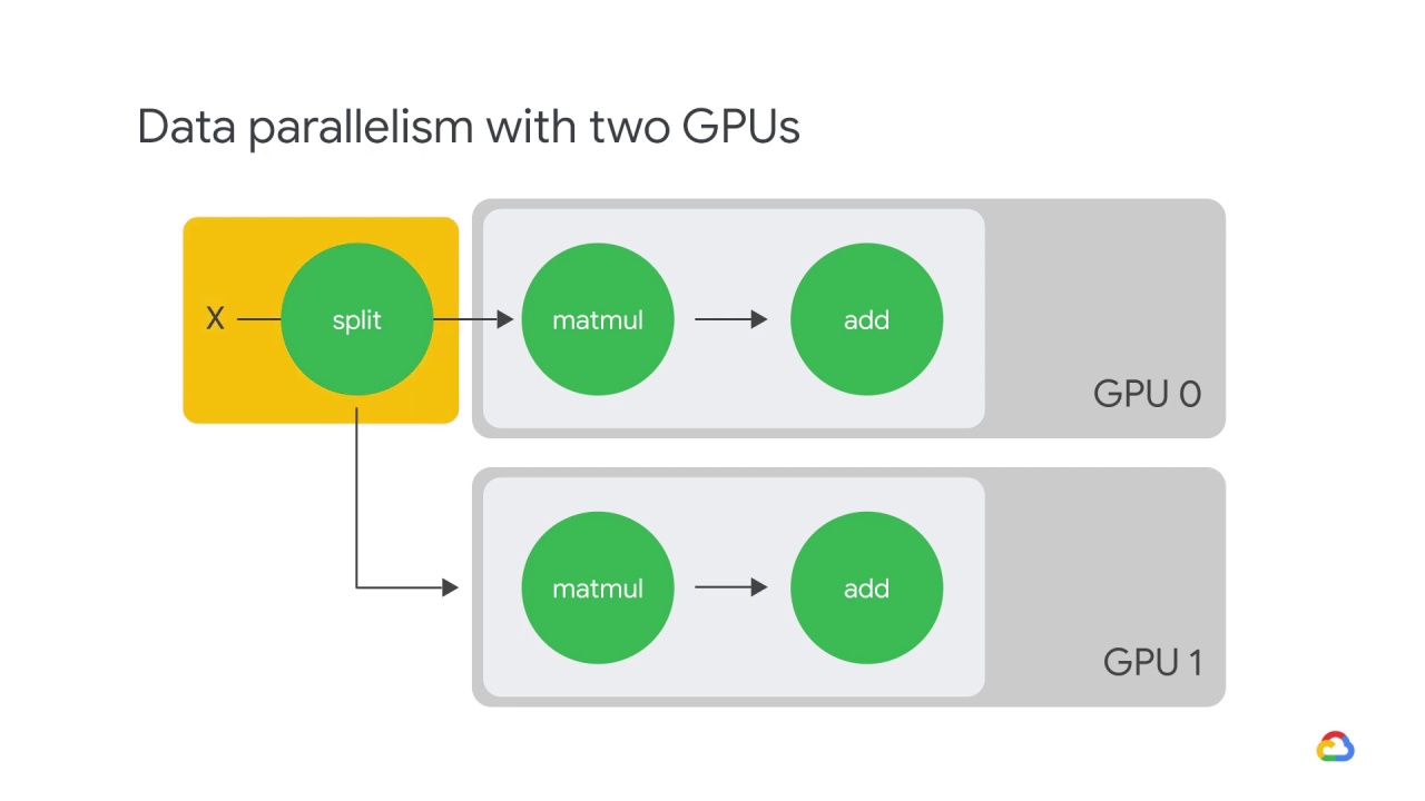
The input batch X is split in half,

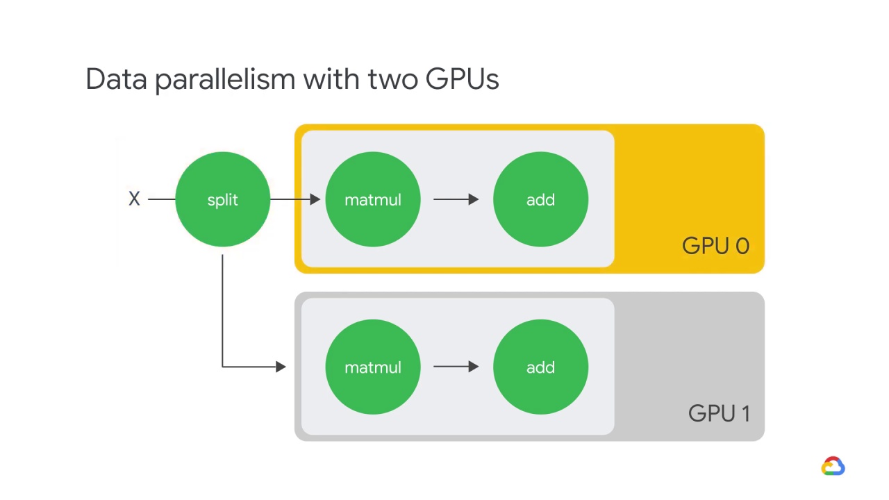
and one slice is sent to GPU 0,

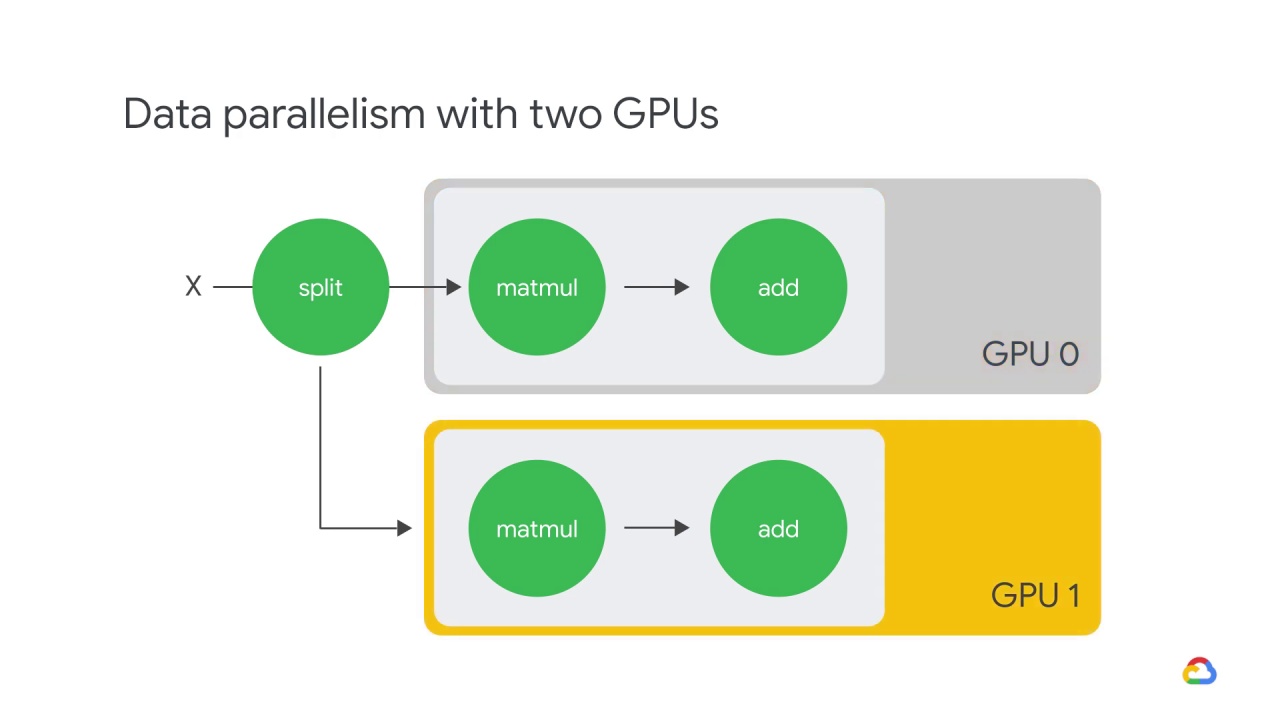
and the other to GPU 1.

In this case, each GPU calculates the same ops but on different slices of the data.

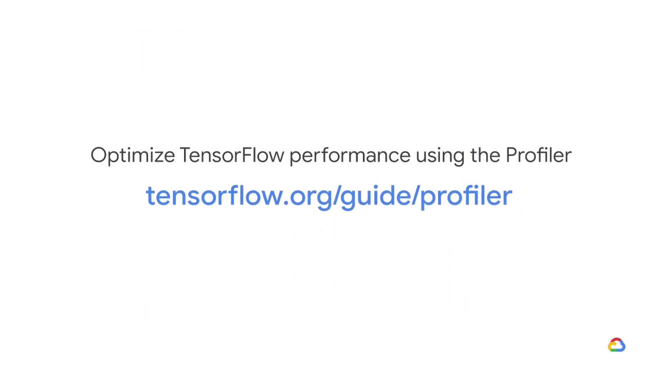
For more information on making the most of your GPUs, please refer to the guide titled, “Optimize TensorFlow GPU Performance with the TensorFlow Profiler,” found at tensorflow.org/guide/gpu_performance_analysis.